 Laboratory
6: Medical Imaging Laboratory
6: Medical Imaging
Coronal
Sections | Horizontal Sections
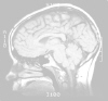
| Sagittal Sections
 Test yourself on the Brainstem
Slides of the Week for Week 6. Test yourself on the Brainstem
Slides of the Week for Week 6.
When you
are finished examining your horizontal and coronal brain slices, turn
to the CT and MR images posted on the light boxes at each end of the
lab. If you have been following the Case
Studies prepared by Dr. Brint, you have already gained considerable
experience in analyzing such images.
X-ray Computed
Tomography (CT) is really a computer-enhanced version of standard
X-ray imaging. Except for dense tissues like bone, visual contrast
is limited (although recent advances in image analysis technology
and the continuing enhancements in computer power have increased the
resolution and visual contrast of CT scans). Usually, you are
only able to discriminate between brain matter and air or fluid-filled
cavities (this is why you need to know the location of ventricles
and cisterns to maintain your orientation). However, as diagnostic
tools go, it is a relatively inexpensive technology and it provides
significant information on the location of pathologies like tumors
or hematomas.
Magnetic
resonance imaging (MRI) has put a new "spin" on the non-invasive
visualization of soft tissue. Atomic nuclei that have an odd
number of protons or neutrons (like hydrogen) will act like tiny magnets,
aligning themselves in strong magnetic fields. When they align
or relax, these nuclei will absorb then give off bursts of electromagntic
energy that can be detected spatially by the detector rings of the
imaging instrument. A computer reconstructs the pattern of electromagnetic
emissions. The pattern ends up looking remarkably like the tissue
being studied!
MRI has
become incredibly important for the study of the normal and pathological
brain. The images are usually derived based on one of two time
constants - TE and TR. Time between the radiofrequency pulse
emited by the machine and the detection of the magnetic signal from
the patient is the TE (echo time). T1 is the time constant with which
nuclei return to alignment with the static magnetic field.
T2 is the time constant with which nuclei, all perturbed at the same
time by the radiofrequency pulse, lose alignment with each other.
You don't need to be a nuclear physicist to appreciate that these
different time constants emphasize different tissue characteristics.
For example, with T1 weighted images (TE < 30 msec), image brightness
is generally proportional to the water and fat content of the tissue:
bone is dark, fat is bright, white matter is light, gray matter is
dark, and air and fluid-filled spaces are near black. With T2
weighted images (TE > 60 msec), white matter is darker than gray
matter, and CSF is bright and prominent (although, where fluid is
flowing, such as in blood vessels and sinuses, the area will appear
dark). TR (the time between pulse repetitions) are usually
optimized for the TE: T1 weighting usually requires a short TR (>
800 msec), T2 images a long TR (> 2000 msce since you are enhancing
for protons with long relaxation times). Our sagittal images are standard
T! weighted images. The horizontal images represent a pair of T1 and
T2 weighted images at each plane of section. However, the T1 images
are unique since the TR was not varied for the pair (TR = 2000 msec
for both T1 and T2 images). This is apparently done to enhance the
signal to noise ratio of T1 rated images and provides a hybrid view
(gray matter is brighter than white matter, but ventricles are dark).
As was demonstrated
in Case Study 1,
imaging parameters can be adjusted to enhance visualization of vessels
and sinuses. Reversing the contrast on such data provides for
extremely high-resolution images that are extremely useful for demonstrating
pathologies in the brain. Taken to the extreme (with a powerful
enough magnet) real time imaging of flow properties can be used to
study dynamic changes in brain responsiveness (functional MRI).
A few examples
of MR images taken from our image set are shown on the following pages
to help you gain your orientation and perspective. Compare
what you see in these images with what you have seen in your wet brain
specimens. Your wet specimens may be your last reminder that
such images represent real, living tissue!
There are
several resources on the Web where you can learn more about Medical
Imaging. One of the better resources is The
Whole Brain Atlas, a marvelous collection of correlated MRIs and
SPECTs from Drs. Keith Johnson and J. Alex Becker at Harvard and MIT.
Check it out! As a reference guide, we used the book: Cardoza, J.D.
and Herfkens, R.J. MRI Survival Guide (1996) Lippincott -
Raven Publishers, Philadelphia/New York.
|